
by Dr. Tao Chen and Dr. Roman Senkov
download this article: pdf (630kb)
Seeing a master at work is always mesmerizing, as if they are performing magic in front of our very eyes. It doesn't matter if we are looking at a culinary chef, a musician, an athlete, or a mathematician. It can be a source of great inspiration. Despite understanding that this magic that we see actually originates from knowledge and years of practice, we're still inspired to pursue their magic ourselves.
In this short article, we will try to demonstrate a few simple, but beautiful mathematical “tricks” and methods, that will allows us to solve quite challenging problems with minimal effort (in this case the problems only appear to be challenging - otherwise they would not have such simple solutions or the hardest part of the solution is somehow hidden). At the end of the article we show how these methods can be applied to some real and not-very-real physics problems.
We hope you'll enjoy the reading and the magic behind equations and formulae. Please feel free to contact us with any questions and, perhaps, solutions.
Tao Chen (tchen@lagcc.cuny.edu),
Roman Senkov (rsenkov@lagcc.cuny.edu)
A series is the sum of infinitely many terms. Usually, adding an infinite amount of terms is a daunting task. Luckily, if these terms have a pattern or they can be derived from a previously derived series the problem becomes manageable. For example, to find
\begin{equation}\tag{1}
S_1(x) =1 + x + x^2 + x^3 + \cdots
\end{equation}
we can rearrange the sum as
\begin{equation}\tag{2}
S_1(x)= 1+x(1 + x + x^2 + x^3 + \cdots).
\end{equation}
We notice that the expression in the brackets is equal to \(S_1(x)\), so we can rewrite the previous equation as
\begin{equation}\tag{3}
S_1(x)=1+x\cdot S_1(x)
\end{equation}
and therefore
\begin{equation}\tag{4}
S_1(x)=1 + x + x^2 + x^3 + \cdots = \frac{1}{1-x}.
\end{equation}
It has to be mentioned that these manipulations require certain conditions such as convergence to be true, that is, the sum of infinitely many terms to be valid (which has to be proven!). Without convergence, the above derivation is not valid. To see the problem try to find \(S_1(x)\) for \(x=1\) or \(x=2\) (actually the sum in Eq.(1) exists only for \(|x| < 1\) ).
The series in Eq.(1) is called a geometric series, but it also helps to find the sum of other series. For example, let
\begin{equation}\tag{5}
S_2(x) = x + \frac{x^2}{2} + \frac{x^3}{3} + \frac{x^4}{4}+ \cdots . \end{equation}
Note that
\begin{equation}\tag{6}
\frac{d S_2(x)}{dx} = 1+x+x^2+x^3+\cdots = S_1(x)
\end{equation}
is a differential equation, \(S'_2(x)=S_1(x)\). Therefore we can integrate it as
\begin{equation}\tag{7}
S_2(x)=\int \frac{1}{1-x}dx = - \ln (1-x).
\end{equation}
Using Eq.(7) we can demonstrate that the following series diverges logarithmically
\begin{equation}\tag{8}
1 + \frac{1}{2} + \frac{1}{3} + \frac{1}{4}+ \cdots = \lim_{x \rightarrow 1} \left[- \ln(1-x)\right] = \infty .
\end{equation}
A similar technique could be applied to find the following famous series
\begin{equation}\tag{9}
S_3(x) = 1 + x + \frac{x^2}{2!} + \frac{x^3}{3!} + \cdots.
\end{equation}
We leave it to the readers: find \(S_3(x)\) and prove that
\begin{equation}\tag{10}
e = 1 + 1 + \frac{1}{2!} + \frac{1}{3!} + \cdots,
\end{equation}where \(e \approx 2.7182818\dots\) is the Euler's number.
Continued fractions are written as fractions within fractions, which are added up in a special way, and which may go on for ever. In fact any fraction can be written as a continued fraction with finite length, such as 11/30 which can be written as
\begin{equation}
\cfrac{1}{2+\cfrac{2}{2+\cfrac{2}{2+\cfrac{2}{3}}}};
\end{equation}
while an irrational number can be written as a continued fraction with infinite length. Similar to a series, continued fractions can be found if there is some pattern. For example, let
\begin{equation}\tag{11}
F_1 = 1+\cfrac{1}{1+\cfrac{1}{1+\cfrac{1}{1+\cfrac{1}{1+\dots}}}}.
\end{equation}
It is easy to see that \[F_1=1+\frac{1}{F_1},\] or \(F_1\) satisfies the equation \(x^2-x-1=0\). Thus \(F_1=\frac{\sqrt{5}+1}{2}\). What happened to the second root of the quadratic equation?
Can you find a more general continued fraction yourself?
\begin{equation}\tag{12}
F_2(x) = x+\cfrac{1}{x+\cfrac{1}{x+\cfrac{1}{x+\cfrac{1}{x+\dots}}}}.
\end{equation}
We can also find more complicated continued fractions, for example, like this one
\begin{equation}\tag{13}
F_3 = 1+\cfrac{1}{2+\cfrac{1}{1+\cfrac{1}{2+\cfrac{1}{1+\dots}}}}.
\end{equation}
Show that \(F_3\) satisfies the following equation
\begin{equation}\tag{14}
F_3 = 1+\cfrac{1}{2+\cfrac{1}{F_3}}
\end{equation}
and find \(F_3\). We leave the solution to diligent readers.
A nested root is a radical expression that contains other radical expressions (nests). Similar to the series and continued fractions, we can also find the precise value of a nested root if it has a certain pattern. For example, let
\begin{equation}\tag{15}
R_1 = \sqrt{2+\sqrt{2+\sqrt{2+ \cdots}}}
\end{equation}
It is easy to see that \(R_1=\sqrt{2+R_1}\). That is, \(R_1\) satisfies the equation \(x^2-x-2=0\). Thus \(R_2=2\). Again, what will happen to the second root of the quadratic equation?
The readers can try to find the following three nested roots:
\begin{equation}\tag{16}
R_2(x) = \sqrt{x+\sqrt{x+\sqrt{x+ \cdots}}}, x\geq 0
\end{equation}
\begin{equation}\tag{17}
R_3 = \sqrt{2- \sqrt{2-\sqrt{2- \cdots}}},
\end{equation}
and
\begin{equation}\tag{18}
R_4 = \sqrt[3]{6+ \sqrt[3]{6+\sqrt[3]{6+ \cdots}}}.
\end{equation}
In this section we consider two physics-related problems. In the first example we calculate the effective resistance of an infinite series of resistors forming an electric circuit. The setup is slightly artificial, but still quite useful to consider, at least from theoretical point of view. The second example is a real-life problem from Quantum Field Theory (QFT). We discuss the idea behind the Schwinger-Dyson equations (SDEs) that involve summation of an infinite number of Feynman diagrams. Quantum field theory in general and SDEs in particular are quite complicated, so we will significantly simplify the problem considering it at a qualitative level.
Consider the electric circuit shown in Fig. 1. One way to find the current through the battery \(V\) is to replace the right-side part of the circuit with an equivalent resistance, \(R_{eq}\).
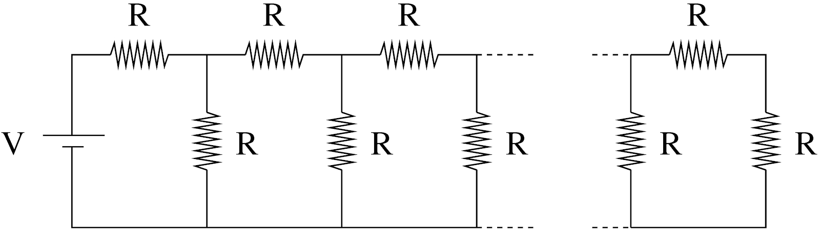
Figure 1: Electric circuit with infinite number of identical resistors.
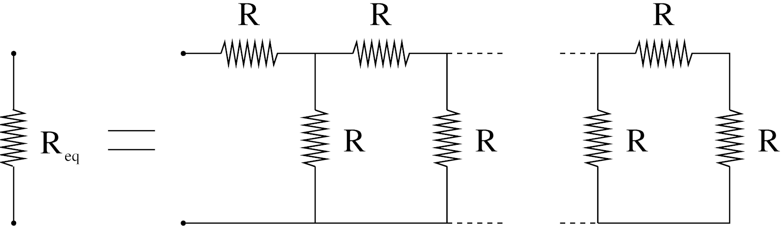
Figure 2: The equivalent resistance.
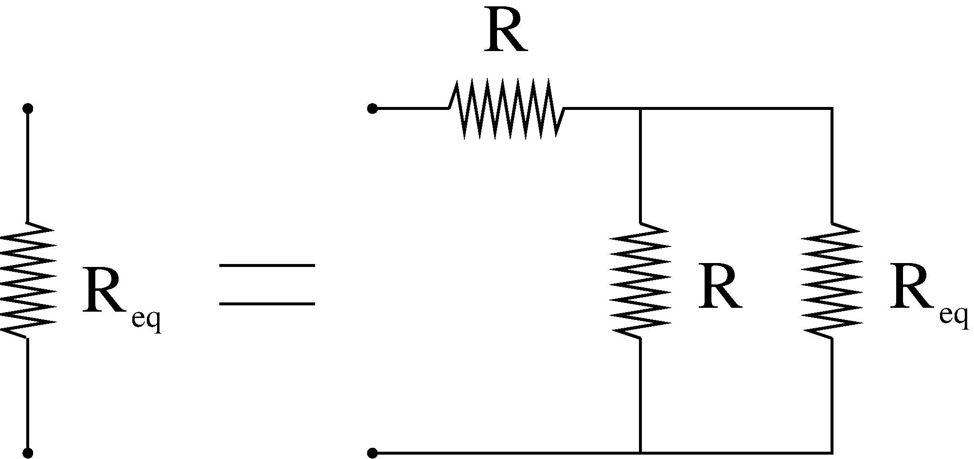
Figure 3: The graphical representation of the equation (19) for the equivalent resistance.
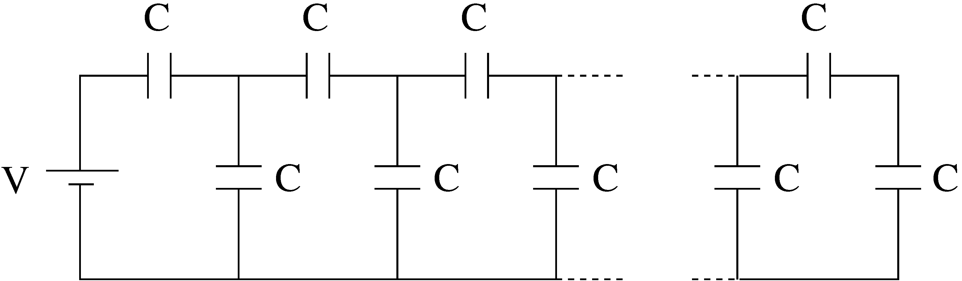
Figure 4: A series of identical capacitors.
In quantum theory we use wave function to describe the probability of finding the particle near certain position or Green's function \(G(x,y)\) which has a similar meaning as the wave function but with the additional condition that initially the particle was at some position \(y\).
The Dyson equation for the single-electron Green's function represented as an infinite series of Feynman diagrams as shown in Fig. 5. As we can see, there are infinite number of possibilities for the electron to reach point \(x\) starting from point \(y\), including free motion (the “bare electron” Green's function \(G_0(x,y)\)) and motion influenced by electromagnetic interaction (“dressed” with various photon exchanges).
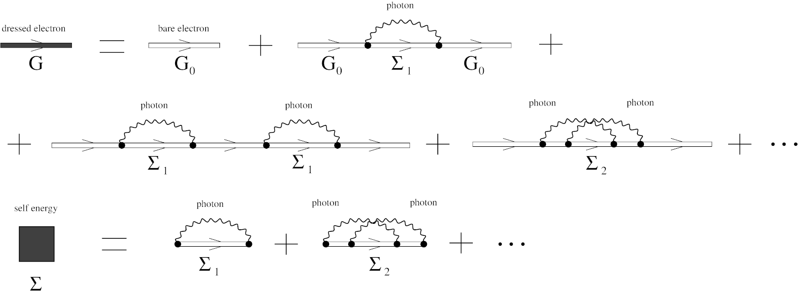
Figure 5: The single-electron Green's function \(G\) and the self-energy operator \(\Sigma\).