
by Dr. Tao Chen (tchen@lagcc.cuny.edu)
In this note, we will review bifurcation patterns of various maps discussed in the literature and introduce a new bifurcation pattern arising in a family of logistic functions.
Populations of people, animals, and items are growing all around us. To describe and predict such changes, scientists and mathematicians use growth models, which provide frameworks for understanding how populations or quantities change over time.
The most basic is linear growth, where the increase is steady and predictable. For example, if a library adds 100 new books each year, starting with 1,000, the collection follows $$N(x)=1000+100x,$$ a straight-line growth pattern.
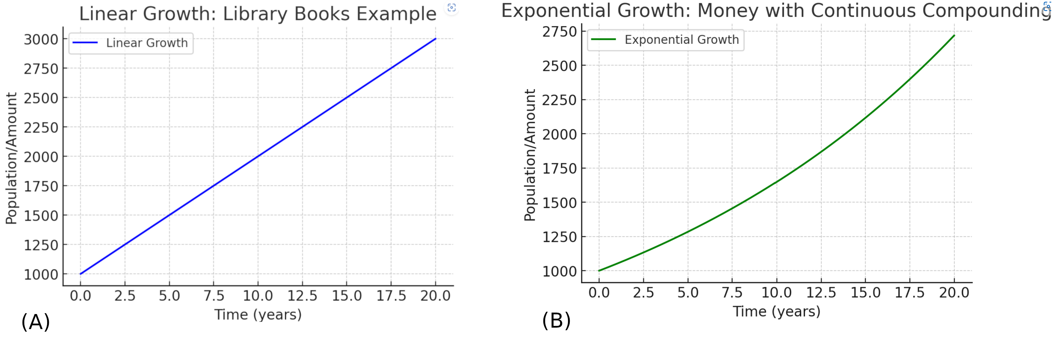
Figure 1. (A) Linear Growth, (B) Exponential Growth.
Exponential growth means that each increase builds on all previous increases. Instead of adding a fixed amount each year, each new increase is calculated from the current total, so the pace of growth keeps accelerating. A classic example is money earning compound interest. If $1,000 is invested at a 5% annual interest rate compounded continuously, the amount after \(t\) years is $$A(t)=1000 e^{0.05t}.$$ The balance grows smoothly and faster over time, reaching about $1,648 after 10 years – much more than the $1,500 from simple linear growth.
Real-world populations, however, rarely grow without limits. Logistic growth models how populations expand in environments with limited resources, such as space and food. As a consequence, populations eventually slow as they approach a maximum sustainable size, called the carrying capacity. For example, imagine a herd of deer in a forest. If the forest can support up to 1,000 deer, which is the carrying capacity, and the herd begins with 50 deer growing at a rate of 0.3 per year, the population grows quickly at first but then gradually stabilizes near 1,000. The logistic growth function is $$f(t)=\frac{1000}{1+19e^{-0.3t}}.$$
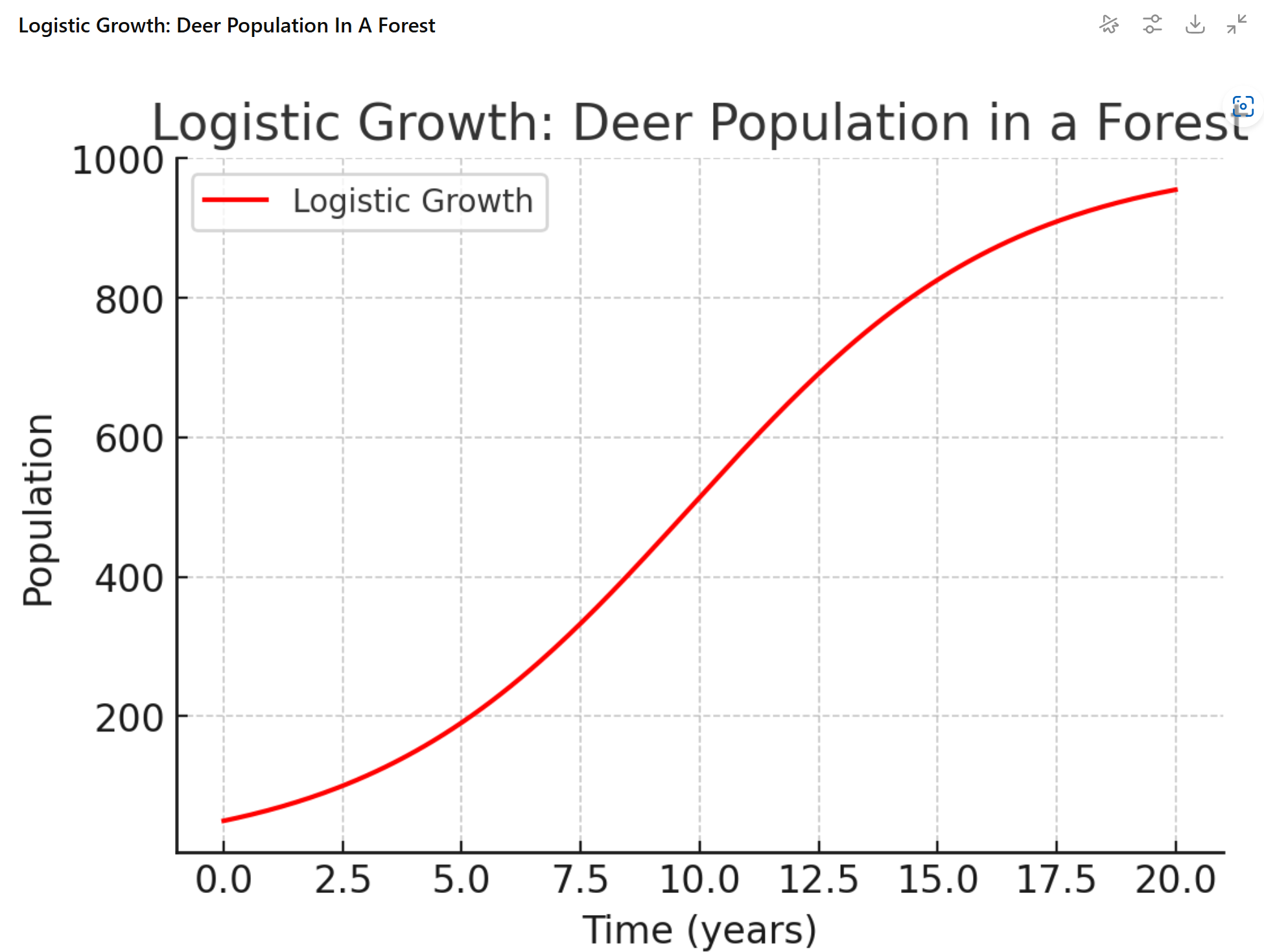
Figure 2. Logistic Growth.
For more details on logistic functions, please check Chapter 4.4 in [7].
In principal, the size of a population in one generation depends directly on the size of the previous generation following one of these growth model, denoted by \(y=f(x)\). If the size of the first generation is \(x_1\), then the second generation is given by \(x_2=f(x_1)\). In turn, the third generation is \(x_3=f(x_2)=f^2(x_1)\), and so on. More generally, the size of the \(n-\)generation is obtained from the rule $$x_n=f(x_{n-1})=f^{n-1}(x_1). $$ This repeated application of the same rule to successive outputs is known as the iteration of functions.
Definition 1. Let \(y=f(x)\) be a function, \(x\) be a number. If there exists an \(n\), such that \(f^n(x)=x\) and \(|(f^n)'(x)|<1\), then \(x\) is called an attracting periodic cycle of period \(n\).
Example: For the function \(f(x)=x^2\), 0 is an attracting period cycle of period 1 (or attracting fixed point) as \(f(0)=0\) and \(f'(0)=0\). For the function \(f(x)=x^2-1\), 0 is an attracting period cycle of period 2 as \(f(0)=-1\) and \(f(-1)=0\), that is \(f^2(0)=0\); and \((f^2)'(0)=0\).
The bifurcation pattern of a family of functions describes how the attracting cycles change as the parameters vary.
The two families of maps $$f_t(x)=x^2+t,\, t\in[-2,\frac{1}{4}]\text{ and } f_t(x)=it\ \tan(x),\, t\in[0,\pi]$$ have been investigated thoroughly.
To the family \(f_t(x)=x^2+t\), in the 1970s, Feigenbaum [5, 6] and independently, Coullet and Tresser [3], discovered an interesting phenomenon called period doubling: if \(f_t\) has an attracting cycle of period \(n\), then the attracting cycle doubles as an attracting cycle of period \(2n\).
(1) For each \(t\in (-3/4, 1/4)\), \(f_t\) has an attracting fixed point.
(2) For each \(t\in (-5/4, -3/4)\), \(f_t\) has an attracting fixed point, and so on.
(3) the period of the attracting cycle follows the pattern $$1\to 2\to 4\to 8\to 16\to 32\to 64\cdots.$$
For the family \(f_t=\it \ \tan(x)\), in [1], we showed that the pattern of bifurcation following cycle merging and cycle doubling: If \(f(t)\) has two attracting cycles of period \(n\), then these two cycles merge into one attracting cycle of period \(2n\) as \(t\) varies; then the one cycle of period \(2n\) is doubled as two attracting cycles of period \(2n\) as \(t\) varies. Specifically, the pattern of bifurcation follows $$(2,4)\to (1,8)\to (2,8)\to (1,16)\to (2,16)\to (1,32)\to (2,32)\to \cdots. $$
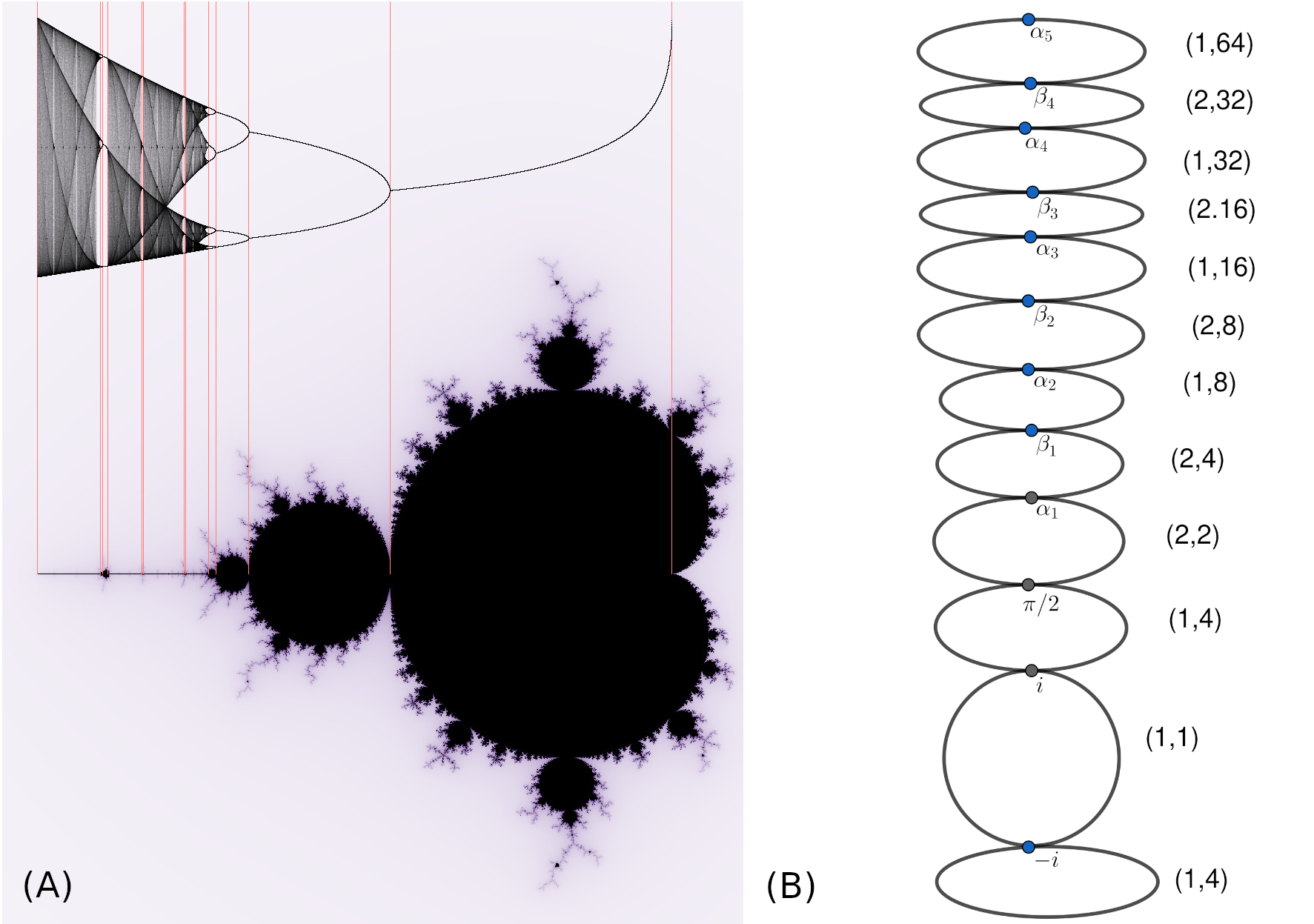
Figure 3. (A) Period Doubling, (B) Cycle Merging and Cycle Doubling.
Recently, in [2], we found a new bifurcation pattern for the family of logistic functions $$f_t(x)=\frac{1}{t+e^{-2x}},t\in(-\infty,\infty).$$ We need some new definitions to describe it.
Definition 2 (Farey Addition, [4]). The Faray sum of two fractions follows $$\frac{a}{b}+\frac{c}{d}=\frac{a+c}{b+d}$$
Definition 3 (Shift of \(n\) points). Let \(f(x)\) has an attracting cycle of period \(n\). If these \(n-\) points are arranged as \(x_1, \cdots, x_n \) from the left to the right. Then there exists a \(k\) such that \(f(x_i)=x_{i+k\mod n}\). Such maps are denoted as \(k/n\).
Example: Suppose a function has \(f\) has a cycle of period 4, denoted by \(x_1, x_2, x_3, x_4\) from the left to the right. If the orbit is \(x_1\mapsto x_2\mapsto x_3\mapsto x_4\mapsto x_1,\) it is denoted as 1/4; while the orbit is \(x_1\mapsto x_4\mapsto x_3\mapsto x_2\mapsto x_1,\) it is denoted as 3/4.
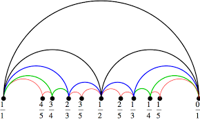
Figure 4. Farey Sequences.
Theorem 2.1. The pattern of bifurcation of the map \(f_t(x)=1/(t+e^{-2x})\) follows Farey sequence. Specifically:
(1) On the most right, the map has an attracting fixed points, denoted by 0/1.
(2) On the most left, the map has an attracting fixed point, denoted by 1/1.
(3) If there exist two maps with \(k_1/m\) and \(k_2/n\) respectively, then there exists a map with \((k_1+k_2)/(m+n)\) in between.
That is, between 0/1 and 1/1, there is a map with an attracting cycle of period 2 with 1/2; between 0/1 and 1/2, there is a map with an attracting cycle of period 3 with 1/3, while between 1/2 and 1/1, there is a map with an attracting cycle of period 3 with 2/3, and so on.
We gratefully acknowledge the Ad Astra Undergraduate Research Newsletter for providing the opportunity to present and summarize our current research. We also wish to thank ChatGPT for its assistance in editing the introduction and generating the graphs. This work was supported by the PSC-CUNY Research Grant Program and the American Mathematical Society–Simons Research Enhancement Grants for Primarily Undergraduate Institution (PUI) Faculty.
[1] T. Chen, Y. Jiang, and L. Keen, “Cycle Doubling, Merging and Renormalization in the Tangent Family,” Conformal Geometry and Dynamics of the American Mathematical Society, 22 (2018), 271–314.
[2] T. Chen, L. Keen, “Farey Tree and Dynamics,” In preparation.
[3] P. Coullet and C. Tresser, “Itérations d'endomorphismes et groupe de renormalisation,” Journal de Physique Colloque C5, Supplément au no. 8, tome 39, août 1978, 5–25.
[4] “Farey Sequences,” Wikipedia, https://en.wikipedia.org/wiki/Farey_sequence.
[5] M. Feigenbaum, “Quantitative universality for a class of non-linear transformations,” Journal of Statistical Physics, 19 (1978), 25–52.
[6] M. Feigenbaum, “The universal metric properties of non-linear transformations,” Journal of Statistical Physics, 21 (1979), 669–706.
[7] G. Strang and E. Herman, Calculus Volume 2, OpenStax (2016). https://openstax.org/details/books/calculus-volume-2/