
by Dr. Frank Wang (fwang@lagcc.cuny.edu)
We use Richard Wagner's literary invention “here time becomes space” in Parsifal to illustrate an intriguing idea in Big-Bang cosmology and inflationary universe: space is infinite because inflation is eternal. Although the connection between music and physics is metaphorical, this exposition is scientific grounded in general relativity and quantum mechanics, as presented in canonical textbooks and peer-reviewed publications.
The title of this essay is the English translation of “zum Raum wird hier die Zeit.” It is taken from the libretto of Parsifal, [1] the last opera by the German composer Richard Wagner (1813 –1883). This line leads to the Transformation Music (Verwandlungsmusik) in Act I. The opera was first performed in 1882 at the Festspielhaus in Bayreuth, a town in northern Bavaria. Before Albert Einstein (1879 –1955), space and time were considered separate. The concept of spacetime, introduced in 1908 by Einstein's professor Hermann Minkowski, was a major conceptual breakthrough in twentieth-century physics. I have been contemplating the possibility that Wagner's idea might have influenced Einstein's thinking, but I have found no evidence for it. In fact, Wagner's music was not particularly favored by Einstein. Nevertheless, Wagner's literary invention can serve as an interesting metaphor for our contemporary understanding of the cosmos.
Modern cosmology is rooted in Einstein's general relativity. John Wheeler summarized it as “geometry tells matter how to move, and matter tells geometry how to curve.” To appreciate Wheeler's dictum, let's examine Einstein's celebrated field equation: [2] \begin{equation}\tag{1} R_{\mu \nu} - \frac{1}{2} g_{\mu \nu} R = 8 \pi G \, T_{\mu \nu}, \end{equation} where \(R_{\mu \nu}\) is the Ricci tensor, \(g_{\mu \nu}\) the metric tensor, \(R\) the Ricci scalar, \(G\) the gravitational constant, and \(T_{\mu \nu}\) the energy-momentum tensor. The speed of light is set as unity and does not appear in the equation. For those interested in the concept rather than the calculation, we can just regard the left-hand side of the equation as curvature and the right-hand side matter and energy.
A review of elementary geometry might be helpful. Most people can recall the Pythagorean Theorem relating the lengths of the sides \(a\), \(b\) and the hypotenuse \(c\) (not the speed of light) of a right triangle: \(a^{2}+b^{2} = c^{2}\). In calculus, students learn how to calculate the arclength of a curve by cutting it into small segments, and the square of the length of each segment is \(\Delta s^{2} = \Delta x^{2} + \Delta y^{2}\). We can just add the lengths of these segments to obtain the approximate arclength. The exact arclength is the integration of the infinitesimal line element, $$ ds^{2} = dx^{2} + dy^{2}, \quad L = \int_{\mathcal{A}}^{\mathcal{B}} ds , $$ where \(\mathcal{A}\) and \(\mathcal{B}\) are end points. In three dimensions, the line element is $$ ds^{2} = dx^{2} + dy^{2} + dz^{2}. $$ Minkowski showed that Einstein's special relativity is best understood in a four-dimensional spacetime, with the line element $$ ds^{2} =- dt^{2} + dx^{2} + dy^{2} + dz^{2} . $$ Note the minus sign in the time component. This line element is independent of the coordinates we choose. Some people like to say that in relativity, everything is relative. They miss the point. While space and time can depend on the observers if they use different coordinate systems, the spacetime interval does not. In Emmy Noether's seminal paper, which laid the foundation for modern physics, she concluded that Einstein's relativity is a “theory of invariance.” [3]
Euclidean geometry is about flat spaces. If we use polar coordinates, the infinitesimal line element can be written as \(ds^{2} = dr^{2} + r^{2} \, d \theta^{2}\). Consider in general $$ ds^{2} = g_{xx} \, dx^{2} + 2 g_{xy} \, dx \, dy + g_{yy} \, dy^{2}, $$ Carl Friedrich Gauss was able to calculate intrinsic curvature of a two-dimensional surface based on the metric tensor elements \(g_{xx}\), \(g_{xy}\) and \(g_{yy}\), a result published in his Theorema Egregium in 1827. Bernhard Riemann extended Gauss's idea and developed Riemannian geometry, which Einstein later adopted. A curved spacetime has the line element $$ ds^{2} = g_{\mu \nu}(x) \, dx^{\mu} dx^{\nu} , $$ where \(\mu\) and \(\nu\) run from 0 to 3. Here the Einstein summation convention is used: when an index variable such as \(\mu\) or \(\nu\) appears twice, it implies summation.
A simple example of a curved spacetime is \begin{equation}\tag{2} ds^{2} = - dt^{2} + a^{2}(t) (dx^{2} + dy^{2} + dz^{2}), \end{equation} and this turned out to be an excellent description of our universe. Historically, Einstein proposed a static isotropic and homogeneous universe shortly after he completed general relativity. The Russian physicist Alexander Friedmann proposed a time-dependent scale factor \(a(t)\), but he was not properly credited for such an important insight even by the Nobel Committee. [4] The time evolution of \(a(t)\) is governed by the Friedmann equation to be discussed below, and the solution is shown in Figure 1.
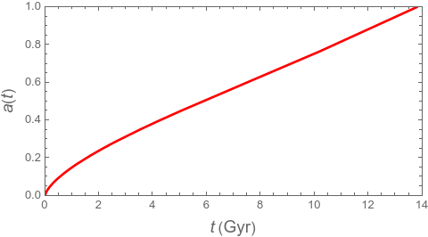
Figure 1: Solution of the Friedmann equation (6) that governs \(a(t)\), with the initial condition is set as \(a(0)=0\). Around \(t \approx 9\) billion years, the concavity of \(a(t)\) changed.
We will set and solve the Friedmann equation in a moment; an important result is that \(a(t)=0\) is possible. When this happens, the metric reduces to \(ds^{2} = - dt^{2}\), representing a state with no spatial dimensions. This is the “Big Bang.” So Wagner's phrase “here time becomes space” can be metaphorically construed as the transformation from a time only metric to the beginning of the Big-Bang cosmology in the context of classical general relativity.
Given a metric tensor \(g_{\mu \nu}\), one can employ Gauss and Riemann's procedure to calculate the curvature tensor. A computer can be programmed to perform such a task, and nowadays physicists routinely use Maple or Mathematica to calculate the curvature tensor. Cosmologists treat the constituents of the universe as a perfect fluid, and according to this approximation we can choose a coordinate system such that the energy-momentum tensor \(T_{\mu \nu}\) is a diagonal matrix consisting of the energy density \(\rho\) and pressure \(p\); they are related through the equation of state. Putting all these together, the Friedmann equation governing \(a(t)\) is \begin{equation}\tag{3} \frac{\dot{a}^{2}}{a^{2}} =\frac{ 8 \pi G}{3} \rho, \end{equation} where \(\dot{a}\) means the derivative of \(a(t)\) with respect to time \(t\). The second derivative of \(a(t)\) satisfies this equation \begin{equation}\tag{4} \frac{\ddot{a}}{a} = -\frac{4 \pi G}{3} (\rho + 3 p). \end{equation} This equation shows that if \(\rho + 3 p\) is negative, gravity can be repulsive, which is crucial in the modern inflationary cosmology we will describe shortly.
In Einstein's original model, he introduced a cosmological constant \(\Lambda\) to make his universe static, and the field equation becomes \begin{equation}\tag{5} R_{\mu \nu} - \frac{1}{2} g_{\mu \nu} R = 8 \pi G \, T_{\mu \nu} + \Lambda g_{\mu \nu}. \end{equation} Although Einstein later regretted modifying his original equation, astronomers in 1998 discovered that the \(\Lambda\) term is indeed needed to explain observational data. The existence of \(\Lambda\) implies \(p=-\rho\), and \(\rho + 3 p = -2 \rho\), meaning repulsive gravity. If you examine Figure 1 carefully, you should notice that about 9 billion years after the Big Bang the concavity of the curve of \(a(t)\) changed, signifying that the universe began to expand at an accelerating rate.
Our universe is currently understood to contain three energy forms: radiation, matter (or “dust”), and dark energy related to the cosmological constant. The equation of state for radiation is \(p = \rho/3\), with \(\rho \propto a^{-4}\). For dust, \(p=0\), and \(\rho \propto a^{-3}\). For dark energy, \(p=-\rho\), and \(\rho\) is constant. Astronomers define the Hubble parameter as $$ H = \frac{\dot{a}(t)}{a(t)}, $$ and the cosmological redshift $$ 1+z = \frac{1}{a(t)}. $$ They use the density parameter $$ \Omega = \frac{8 \pi G}{3 H^{2}} \rho $$ to express the Friedmann equation in terms of measurable quantities, $$ \frac{\dot{a}^{2}}{a^{2}} = H_{0}^{2}( \Omega_{\mathrm{v}} + \Omega_{\mathrm{m}} a^{-3} + \Omega_{\mathrm{r}} a^{-4}), $$ where \(H_{0}\) is \(H\) at the present time, \(H_{0} = 1/14.507\) Gyr\(^{-1}\), and values of density parameters are \(\Omega_{\mathrm{m}}=0.315\) (matter), \(\Omega_{\mathrm{v}}=0.685\) (dark energy), \(\Omega_{\mathrm{r}}= \Omega_{\mathrm{m}}/(1+z_{\mathrm{eq}}) = 9.26 \times 10^{-5}\) (radiation). [5] The Friedmann equation can be integrated numerically, \begin{equation}\tag{6} t(z) = \frac{1}{H_{0}} \int_{0}^{1/(1+z)} \frac{dx}{x \sqrt{\Omega_{\mathrm{v}} + \Omega_{\mathrm{m}} x^{-3} + \Omega_{\mathrm{r}} x^{-4}}} , \end{equation} and this is the solution shown in Figure 1. In this integral, we define the zero of time as corresponding to an infinite redshift \(z \rightarrow \infty\). A striking implication of relativistic cosmology is that, according to this model, the universe has not existed forever. We can write the above as an improper integral $$ t_{0} \equiv \lim_{z \rightarrow \infty} t(z) = \frac{1}{H_{0}} \int_{0}^{\infty} \frac{dz}{(1+z) \sqrt{\Omega_{\mathrm{v}} + \Omega_{\mathrm{m}} (1+z)^{3} + \Omega_{\mathrm{r}} (1+z)^{4}}} , $$ and it converges to 13.8 billion years, despite the upper limit of infinity. This is referred to as the age of the universe. By convention, the moment of the Big Bang, \(a(t)=0\), is defined as \(t=0\). This choice is arbitrary, similar to the designation of “AD” (anno Domini) in the Gregorian calendar, but without religious implication.
A side story: Georges Lemaître, Belgian Catholic priest and astronomer, is often credited as the father of the Big Bang theory. He received his Ph.D. from MIT in 1927, and he was the first to connect Edwin Hubble's astronomical observations to Einstein's general relativity. Based on the finite age of the universe, Lemaître wrote a paper titled “The Beginning of the World from the Point of View of Quantum Theory” and proposed that the universe expanded from a single initial quantum, which he called the “primeval atom.” [6] Initially Einstein was very negative about Lemaître's physics, but eventually Einstein embraced Lemaître's ideas. The moral is that even Einstein did not realize his own general relativity's predictive power.
The standard Big-Bang model provides a successful framework for understanding the thermal history of our universe. However, the observed high degree of isotropy in the cosmic microwave background radiation presents a puzzle, known as the horizon problem. The metric in Eq. (2) describes a spatially flat universe, but such a configuration is unstable – this is known as the flatness problem. In 1981, Alan Guth proposed an earlier period of inflation, during which the universe's energy density was dominated by a slowly varying vacuum energy, causing \(a(t)\) to grow approximately exponentially. Inflation theory solves several major problems in the Big-Bang cosmology. [7]
In his treatise Cosmology, [8] Steven Weinberg described the current mainstream cosmology as a scenario according to which inflation driven by one or more scalar fields followed by a Big Bang dominated by radiation, cold dark matter, baryonic matter, and vacuum energy. As Columbia University professor Brian Greene put it, rather than inflation being incorporated into the standard Big Bang theory, the standard Big Bang would be incorporated into inflation. [9]
The simplest possibility to generate an accelerating expansion is through a scalar field. At least one such field is known to exist: the Higgs field. A typical Lagrangian density is \begin{equation}\tag{7} \mathcal{L} = -\frac{1}{2} g^{\mu \nu} \frac{\partial \phi}{\partial x^{\mu}} \frac{\partial \phi}{\partial x^{\nu}} -V(\phi) . \end{equation} Using Noether's theorem, [3] the elements of \(T_{\mu \nu}\) can be found as [8] \begin{equation}\tag{8} \rho = -\frac{1}{2} g^{\mu \nu} \frac{\partial \phi}{\partial x^{\mu}} \frac{\partial \phi}{\partial x^{\nu}} +V(\phi) , \end{equation} \begin{equation}\tag{9} p = -\frac{1}{2} g^{\mu \nu} \frac{\partial \phi}{\partial x^{\mu}} \frac{\partial \phi}{\partial x^{\nu}} -V(\phi) , \end{equation} while the 4-velocity is proportional to the gradient of the field, \(u^{\mu} \propto \nabla^{\mu} \phi\), or explicitly \begin{equation}\tag{10} u^{\mu} = - \left[-g^{\rho \sigma} \frac{\partial \phi}{\partial x^{\rho}} \frac{\partial \phi}{\partial x^{\sigma}} \right]^{-1/2} g^{\mu \tau} \frac{\partial \phi}{\partial x^{\tau}} . \end{equation} If the scalar field is uniform in time and space, then \(p=-\rho = -V(\phi)\), resembling Einstein's cosmological constant, which can drive exponential expansion. It is commonly assumed that the potential \(V(\phi)\), such as the one shown in Figure 2, will lead to a slow-roll inflation, which ended with a period of reheating when the scalar field \(\phi\) decayed into particles and thermalized to recover a hot Big-Bang cosmology at the end of inflation. [10] The MIT professor Max Tegmark wrote “what we've called our Big Bang wasn't the ultimate beginning, but rather the end of inflation in our part of space.” [11]

Figure 2: The Starobinsky model of inflation potential, with \(M\) the scalar field mass, \(\displaystyle{V(\phi) = \frac{3}{4} M^{2} \left(1-e^{-\sqrt{2/3} \, \phi} \right)^{2}}\). This potential has the same form as the Morse potential for a diatomic molecule.
If the inflaton scalar field at a given point in space once had a value of unstable equilibrium (like at the top of a potential hill), then the probability that the inflation field was still at this value after a time \(t\) decreased as \(\exp(-\gamma t)\) where \(\gamma\) is the decay constant. However, the volume in which the scalar had this value was meanwhile increasing as \(\exp(+3Ht)\), where \(\displaystyle{H = \sqrt{\frac{8 \pi G}{3}\left(\frac{1}{2} \dot{\phi}^{2} + V(\phi)\right)}}\). As long as \(3H > \gamma\), the volume of space that still undergoes inflation increases exponentially. Such a scenario is “eternal inflation.” [8] In Andrei Linde's theory of “chaotic inflation,” initially one or more scalar fields varied in a random way with position. [12] Here and there one would have found patches of space in which an inflaton field took a nearly uniform value, and inflation will then have occurred in such a patch, provided the patch was initially sufficiently large, much greater than the Planck length, \(1.616 \times 10^{-35}\) meters. Such relatively large uniform patches may be quite rare, but there is no argument against this hypothesis. The patch will grow to an enormous size eternally. When the scalar field evolves towards the minimum of its potential shown in Figure 2, the energy density locked in the potential energy of the field is converted to kinetic energy, a process called reheating mentioned earlier, although there was not necessarily any preceding thermal era. Reheated bubbles can be produced endlessly, and in most models, they do not percolate. These causally disconnected bubble universes constitute a “multiverse.” [5] Our observable universe is supposed to occupy a small part of one such bubble.
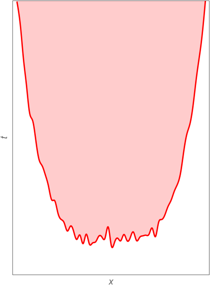
Figure 3: The spacetime structure of one of the bubble universes. Inflating region is white, and thermalized region is shaded; the boundary is the Big Bang. While the boundary appeared time-like at large \(t\), it is an infinite spacelike hypersurface with an appropriate choice of coordinates, see Eq. (10). Eternal time becomes infinite space in this picture.
A spacetime slice outside one of the bubble universe is shown in Figure 3. The thermalization hypersurface with constant \(\phi\) is schematically shown as the red curve, and the wiggling is caused by quantum fluctuations. Such a hypersurface plays the role of the Big Bang for the corresponding thermalized regions indicated by the shaded areas. The surfaces \(\phi=\)constant are spacelike, thus the value of \(\phi\) can be used to define as “time” inside a bubble Universe. In general, thermalization hypersurfaces cannot terminate. [13], [14] In Brian Greene's description, [15] what appears an endless time to an outsider appears as endless space, at each moment of time, to an insider. This reminds us of Wagner again: “here time becomes space” on the Big-Bang hypersurface.
The Tufts University cosmologist Alexander Vilenkin wrote a popular book Many Worlds in One, [16] which is based on his Physical Review paper of the same title. The consequence of a spatially infinite universe is that it contains an infinite number of regions of the same size as our observable universe, which he called \(\mathcal{O}\) regions. The number of possible histories which may take place inside an \(\mathcal{O}\) region is finite. Hence, all histories which are not forbidden by physics will occur in a finite fraction of all \(\mathcal{O}\) regions. To summarize Vilenkin's theory, the number of possible histories is finite, but the universe is infinite, thus every possible history occurs an infinite number of times.
I thank Dr. Roman Senkov and Amaru Alzogaray for their valuable suggestions for improving this paper. I thank Dr. Ali Erginay for taking the pictures at the Bayreuth Festspielhaus.
[1] Richard Wagner, Parsifal: ein Bühnenweihfestspiel, B. Schott's Söhne, Mainz, 1877. The English translation by Stewart Robb (Schirmer) of the stage direction for the Act I Transformation Music is the following. As Parsifal and Gurnemanz appear to walk, the scene changes more and more visibly. The forest disappears and a doorway appears in rocky walls concealing the two. The two enter the vast hall of the Grail castle. We see a pillared hall with a high dome in the center over the reflectory. Enter the knights of the Grail, who take their places at the tables. On Christmas Eve in 1903, the Metropolitan Opera in New York defied the wishes of Cosima Wagner, the composer's widow, by staging the first performance of Parsifal outside of Bayreuth. The production was featured in the cover story in the February 6, 1904 issue of Scientific American.
[2] C. W. Misner, K. S. Thorne, J. A. Wheeler, Gravitation, Freeman, San Francisco, 1973.
[3] Emmy Noether, “Invariante Variationsprobleme.” Nachrichten von der Gesellschaft der Wissenschaften zu Göttingen, Mathematisch-Physikalische Klasse, 235–257 (1918). See the English translation, https://arxiv.org/abs/physics/0503066, the last footnote.
[4] Ari Belenkiy, “Alexander Friedmann and the Origins of Modern Cosmology,” Physics Today, 38–43, October 2012.
[5] K. A. Olive and J. A. Peacock, “Big-Bang Cosmology,” in S. Navas et al. (Particle Data Group), Physical Review, D 110, 030001 (2024).
[6] G. Lemaître, “The Beginning of the World from the Point of View of Quantum Theory,” Nature, 127, 706 (1931).
[7] Alan H. Guth, “Inflationary Universe: A Possible Solution to the Horizon and Flatness Problems,” Physical Review, D 23, 347–356 (1981). The possibility of an early exponential expansion of the universe had been noticed by several Russian authors around 1980.
[8] Steven Weinberg, Cosmology, Oxford University Press, Oxford, 2008.
[9] Brian Greene, The Fabric of the Cosmos, Knopf, New York, 2004, p. 321.
[10] J. Ellis and D. Wands, “Inflation,” in S. Navas et al. (Particle Data Group), Physical Review, D 110, 030001 (2024).
[11] Max Tegmark, Our Mathematical Universe, Knopf, New York, 2014, p. 113.
[12] Andrei Linde, Dmitri Linde, and Arthur Mezhlumian, “From the Big Bang Theory to the Theory of a Stationary Universe,” Physical Review, D 49, 1783–1826 (1994).
[13] Vitaly Vanchurin, Alexander Vilenkin, and Serge Winitzki, “Predictability Crisis in Inflationary Cosmology and Its Resolution,” Physical Review, D 61, 083507 (2000).
[14] Jaume Garriga and Alexander Vilenkin, “Many Worlds in One,” Physical Review, D 64, 043511 (2001).
[15] Brian Greene, The Hidden Reality, Knopf, New York, 2011, p. 79.
[16] Alexander Vilenkin, Many Worlds in One, Hill and Wang, New York, 2006.