
by Zane Avan
This work was done by LaGuardia student Zane Avan as part of the Honors “General Physics I” class, Fall 2024. In this work, Zane studies how the Moon slightly perturbs the Earth’s orbit around the Sun and estimates the resulting precession of the Earth’s perihelion.
The research was conducted under the supervision of Dr. Roman Senkov.
Other research projects done by students in the Physics Honors courses: “Maupertuis's Principle and Its Analog in Quantum Mechanics”, “Orbital Decay of a Massive Black Hole”, “Atomic Nuclei and Pairing Correlations”, “Lagrange Points in Binary Star Systems”, and “Unveiling Stellar Dimensions: An Exploration of Neutron Stars and White Dwarfs”.
Download this article: pdf (220K)
We study the influence of the Moon on the Earth's orbit around the Sun. Starting from the Newtonian gravitational interaction in the Sun–Earth–Moon system, we use the mass hierarchy of the Sun–Earth–Moon system to derive a correction to the effective Earth–Sun potential energy. In the absence of this correction, and neglecting other perturbations, the Earth's motion reduces to the standard Kepler problem and the orbit is an ellipse. The Moon-induced correction causes a small deviation from this ideal Keplerian motion, leading to a gradual precession of the Earth's perihelion. We estimate this precession to be approximately 7.9 arcseconds per century and compare it with other known contributions to the Earth's orbital precession.
The motion of the Earth around the Sun is often described as a two-body Kepler problem. In this approximation, the Earth follows an elliptical orbit with the Sun located at one focus [1]. This model provides an excellent first description of planetary motion, but it neglects several smaller effects that perturb the orbit. These include gravitational interactions with other planets, especially massive planets such as Jupiter, as well as corrections from Einstein’s general theory of relativity.
Small deviations from ideal Keplerian motion have long played an important role in gravitational physics. A famous example is the anomalous precession of Mercury’s orbit, which could not be fully explained by Newtonian gravity and became one of the early successes of general relativity. More broadly, orbital precession can reveal the influence of additional physical effects, including gravitational perturbations from nearby bodies, relativistic corrections, or extra sources of mass.
In this work, we focus on one specific Newtonian perturbation: the gravitational influence of the Moon on the motion of the Earth–Moon system around the Sun. As the Moon orbits the Earth, its distance from the Sun changes slightly. When the Moon is closer to the Sun, it experiences a somewhat stronger solar gravitational force; when it is farther away, this force is weaker. This difference produces a small perturbation of the Earth–Moon system and contributes to the precession of Earth’s orbit around the Sun.
The Earth–Moon–Sun system has a natural hierarchy in both masses and distances, with the Sun far more massive than the Earth and the Earth far more massive than the Moon. This hierarchy allows the Moon’s influence to be treated as a small correction to the dominant Keplerian motion around the Sun. The relevant mass hierarchy is \begin{equation}\tag{1} M_\odot \gg M_{\mathrm{Earth}} \gg M_{\mathrm{Moon}}. \end{equation} Together with the hierarchy of orbital distances, this approximation makes it possible to estimate the Moon-induced precession of the Earth’s orbit around the Sun. Such calculations are also useful more broadly, since accurate models of orbital motion are important for studying planetary systems beyond our own, including Earth-like planets orbiting other stars.
In this section, we develop the theoretical framework used to estimate the precession of the Earth’s orbit due to the Moon. We begin with the standard one-body Kepler problem, which describes the motion of a small mass in the gravitational field of a much heavier body. This provides the unperturbed reference orbit. We then introduce the Moon as a small perturbation and derive the corresponding correction to the effective Earth–Sun potential energy. Finally, we use this correction to estimate the resulting orbital precession.
The standard results about Keplerian motion used in this section follow Ref.[1]; additional references will be given where needed.
Before considering the Moon’s perturbation, we first review the pure Kepler problem: the motion of a body of mass \(m\) in the gravitational field of a much heavier body of mass \(M\). For the Earth–Sun system, the gravitational potential energy is \begin{equation}\tag{2} U(r) = -\frac{\alpha}{r}, \alpha = GMm, \end{equation} where \(r\) is the Earth–Sun distance and \(G\) is the gravitational constant. Since the angular momentum \(L\) is conserved, the radial motion can be described using the effective potential \begin{equation}\tag{3} U_{\mathrm{eff}}(r) = -\frac{\alpha}{r} + \frac{L^2}{2mr^2}. \end{equation} The first term represents the gravitational attraction, while the second term is the centrifugal contribution associated with angular motion.
To determine whether the orbit precesses, we calculate the total angular displacement during one radial cycle, from perihelion to aphelion and back: \begin{equation}\tag{4} \Delta \varphi = \oint d\varphi = 2 \int_{r_{\min}}^{r_{\max}} \frac{d\varphi}{dr} \, dr = 2 \int_{r_{\min}}^{r_{\max}} \left(\frac{\dot{\varphi}}{\dot{r}}\right) \, dr, \end{equation} where \(\dot{\varphi}\) and \(\dot{r}\) are the angular and radial velocities, respectively. From conservation of angular momentum and energy, \begin{align}\tag{5} \dot{\varphi} &= \frac{d \varphi}{dt} = \frac{L}{m r^2}, \\ \dot{r} &= \frac{dr}{dt} = \sqrt{\frac{2}{m} \left(E - U_{\mathrm{eff}}(r)\right)}. \end{align}
The radial turning points, \(r_{\min}\) and \(r_{\max}\), are determined by \begin{equation}\tag{6} E = U_{\mathrm{eff}}(r). \end{equation} They correspond to the closest and farthest points from the Sun, called perihelion and aphelion. Substituting the expressions for \(\dot{\varphi}\) and \(\dot{r}\) gives \begin{equation}\tag{7} \Delta \varphi = 2\int_{r_{\min}}^{r_{\max}} \frac{L}{m r^2} \frac{dr}{\sqrt{\frac{2}{m}\left(E-U_{\mathrm{eff}}(r)\right)}}. \end{equation}
For the effective Kepler potential in Eq. (3), this integral gives \begin{equation}\tag{8} \Delta \varphi = 2\pi. \end{equation} The details of this integration are shown in the Appendix A.1. Thus, after one complete radial cycle, the orbit returns to its original orientation. The pure Kepler orbit is therefore closed and does not precess. Any deviation from \(\Delta \varphi = 2\pi\) indicates orbital precession.
We now derive the correction to the effective Earth–Sun potential caused by the Moon. The Newtonian potential energy of the Sun–Earth–Moon system is \begin{equation}\tag{9} U= -G\frac{M_\odot M_M}{r_1} -G\frac{M_\odot M_E}{r_2} -G\frac{M_E M_M}{r}, \end{equation} where \(M_\odot\), \(M_E\), and \(M_M\) are the masses of the Sun, Earth, and Moon, respectively. Here \(r_1\) is the Sun–Moon distance, \(r_2\) is the Sun–Earth distance, and \(r\) is the Earth–Moon distance, as shown in Fig. 1.
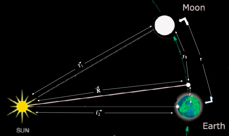
Figure 1: The Sun–Earth–Moon system.
Let \(\vec{R}\) be the position of the Earth–Moon center of mass relative to the Sun. We write the positions of the Moon and Earth relative to the Sun as \begin{equation}\tag{10} \vec{r}_1 = \vec{R}+\vec{r}_3, \qquad \vec{r}_2 = \vec{R}+\vec{r}_4, \end{equation} where \(\vec{r}_3\) and \(\vec{r}_4\) are measured from the Earth–Moon center of mass to the Moon and Earth, respectively. By definition of the center of mass, \begin{equation}\tag{11} M_E\vec{r}_4+M_M\vec{r}_3=0. \end{equation}
The system has a natural hierarchy of masses and distances, \begin{equation}\tag{12} M_M \ll M_E \ll M_\odot, \qquad r_4 \ll r_3 \ll R. \end{equation} Since \(r_3/R\ll 1\) and \(r_4/R\ll 1\), the Sun–Moon and Sun–Earth interactions can be expanded in powers of these small ratios. For example, the Sun–Moon interaction becomes \begin{equation}\tag{13} U_{S-M} = -G\frac{M_\odot M_M}{|\vec{R}+\vec{r}_3|} = -G\frac{M_\odot M_M}{R} \frac{1}{\sqrt{1+ 2\frac{\vec{R}\cdot\vec{r}_3}{R^2} + \frac{r_3^2}{R^2}}}. \end{equation}
Expanding to second order in \(r_3/R\), we obtain \begin{equation}\tag{14} U_{S-M} \approx -G\frac{M_\odot M_M}{R} \left[ 1 -\frac{\vec{R}\cdot\vec{r}_3}{R^2} -\frac{r_3^2}{2R^2} +\frac{3(\vec{R}\cdot\vec{r}_3)^2}{2R^4} \right]. \end{equation} Similarly, for the Sun–Earth interaction, \begin{equation}\tag{15} U_{S-E} \approx -G\frac{M_\odot M_E}{R} \left[ 1 -\frac{\vec{R}\cdot\vec{r}_4}{R^2} -\frac{r_4^2}{2R^2} +\frac{3(\vec{R}\cdot\vec{r}_4)^2}{2R^4} \right]. \end{equation}
Adding Eqs. (14) and (15), we can separate the result into the Kepler term and corrections: \begin{equation}\tag{16} U_{S-E}+U_{S-M} = -G\frac{M_\odot(M_E+M_M)}{R} +\delta U_1+\delta U_2. \end{equation} Here \(\delta U_1\) contains the first-order terms and \(\delta U_2\) contains the second-order terms. The first-order correction is \begin{equation}\tag{17} \delta U_1 = G\frac{M_\odot}{R^3} \left[ M_E(\vec{R}\cdot\vec{r}_4) + M_M(\vec{R}\cdot\vec{r}_3) \right]. \end{equation}
Using the center-of-mass condition in Eq. (11), we find \begin{equation}\tag{18} \delta U_1=0. \end{equation} Thus, the dipole correction cancels, and the leading correction is the second-order, or quadrupole, term: \begin{equation}\tag{19} \delta U_2 = G\frac{M_\odot}{2R^3} \left[ M_E \left( r_4^2 - 3\frac{(\vec{r}_4\cdot\vec{R})^2}{R^2} \right) + M_M \left( r_3^2 - 3\frac{(\vec{r}_3\cdot\vec{R})^2}{R^2} \right) \right]. \end{equation}
We now express \(\vec{r}_3\) and \(\vec{r}_4\) in terms of the Earth–Moon separation vector \(\vec{r}\). If \(\vec{r}\) points from Earth to the Moon, then \begin{equation}\tag{20} \vec{r}_3 = \frac{M_E}{M_E+M_M}\vec{r}, \qquad \vec{r}_4 = -\frac{M_M}{M_E+M_M}\vec{r}. \end{equation} Substituting these expressions into Eq. (19) gives \begin{equation}\tag{21} \delta U_2 = G\frac{M_\odot \mu}{2R^3} \left[ r^2 - 3\frac{(\vec{r}\cdot\vec{R})^2}{R^2} \right], \end{equation} where \begin{equation}\tag{22} \mu=\frac{M_E M_M}{M_E+M_M} \end{equation} is the reduced mass of the Earth–Moon system.
The last term in Eq. (9), \begin{equation}\tag{23} -G\frac{M_E M_M}{r}, \end{equation} describes the internal Earth–Moon interaction. Since this term does not depend on \(R\), it does not affect the motion of the Earth–Moon center of mass around the Sun. Therefore, for the effective Earth–Sun motion, we can omit this internal term.
The effective potential for the Earth–Moon system moving around the Sun is then \begin{equation}\tag{24} U_{\mathrm{eff}}(R) = -G\frac{M_\odot(M_E+M_M)}{R} + G\frac{M_\odot \mu}{2R^3} \left[ r^2 - 3\frac{(\vec{r}\cdot\vec{R})^2}{R^2} \right]. \end{equation}
In this approximation, we treat the Moon’s orbit as circular and, to simplify this expression, we average the quadrupole correction over the Moon’s orbit around the Earth. Writing \begin{equation}\tag{25} \vec{r}\cdot\vec{R}=rR\cos\theta, \end{equation} we have \begin{equation}\tag{26} \left\langle r^2 - 3\frac{(\vec{r}\cdot\vec{R})^2}{R^2} \right\rangle = \left\langle r^2-3r^2\cos^2\theta \right\rangle. \end{equation}
Using \begin{equation}\tag{27} \langle \cos^2\theta \rangle = \frac{1}{2\pi}\int_0^{2\pi}\cos^2\theta\,d\theta = \frac{1}{2}, \end{equation} we obtain \begin{equation}\tag{28} \left\langle r^2-3r^2\cos^2\theta \right\rangle = -\frac{1}{2}r^2. \end{equation}
Therefore, the averaged effective potential becomes \begin{equation}\tag{29} U_{\mathrm{eff}}(R) = -G\frac{M_\odot(M_E+M_M)}{R} - \frac{G M_\odot \mu r^2}{4R^3}. \end{equation} The first term is the usual Kepler potential for the motion of the Earth–Moon system around the Sun. The second term is the Moon-induced correction, \begin{equation}\tag{30} \delta U(R)=-\frac{\beta}{R^3}, \qquad \beta=\frac{G M_\odot \mu r^2}{4}. \end{equation} This correction modifies the pure Kepler problem and leads to a small precession of the Earth’s orbit. In the limit \(M_M\ll M_E\), the reduced mass satisfies \(\mu\approx M_M\), giving the simpler approximation \begin{equation}\tag{31} \beta \approx \frac{G M_\odot M_M r^2}{4}. \end{equation}
We now use the Moon-induced correction derived in the previous section to calculate the corresponding precession of the Earth’s orbit. The averaged correction has the form \begin{equation}\tag{32} \delta U(R)=-\frac{\beta}{R^3}, \qquad \beta=\frac{G M_\odot \mu r^2}{4}, \end{equation} where \(R\) is the distance from the Sun to the Earth–Moon center of mass, \(r\) is the Earth–Moon distance, and \(\mu\) is the reduced mass of the Earth–Moon system. Compared with the pure Kepler problem, this introduces an additional small term proportional to \(1/R^3\).
As before, the total angular displacement during one radial cycle is \begin{equation}\tag{33} \Delta \varphi = 2\int_{R_{\min}}^{R_{\max}} \left(\frac{\dot{\varphi}}{\dot{R}}\right)\,dR, \end{equation} where \(R_{\min}\) and \(R_{\max}\) are the perihelion and aphelion distances, respectively. Using conservation of angular momentum and energy, we obtain \begin{equation}\tag{34} \Delta \varphi = 2\int_{R_{\min}}^{R_{\max}} \frac{L}{mR^2} \frac{dR}{ \sqrt{ \frac{2}{m} \left( E-\frac{L^2}{2mR^2} +\frac{\alpha}{R} +\frac{\beta}{R^3} \right) }}, \end{equation} where \begin{equation}\tag{35} m=M_E+M_M, \qquad \alpha=G M_\odot m. \end{equation}
For \(\beta=0\), Eq. (34) reduces to the pure Kepler result, \(\Delta\varphi=2\pi\). Therefore, any correction to this value represents orbital precession. For small \(\beta\), we write \begin{equation}\tag{36} \Delta \varphi = 2\pi+\delta\varphi, \end{equation} where \(\delta\varphi\) is the precession angle per orbit. Expanding the integral to first order in \(\beta\) gives \begin{equation}\tag{37} \delta\varphi = \frac{6\pi m^2\alpha\beta}{L^4}. \end{equation} The details of this perturbative calculation are given in the Appendix A.2.
This result can be written more transparently using the semi-latus rectum \(p\) of the unperturbed Kepler orbit. For an ellipse, \begin{equation}\tag{38} p=\frac{b^2}{a}=a(1-e^2), \end{equation} where \(a\) is the semi-major axis, \(b\) is the semi-minor axis, and \(e\) is the eccentricity. In orbital mechanics, \(p\) is also related to the angular momentum by \begin{equation}\tag{39} p=\frac{L^2}{m\alpha}. \end{equation}
Using this relation, Eq. (37) becomes \begin{equation}\tag{40} \delta\varphi = \frac{6\pi\beta}{\alpha p^2}. \end{equation} Substituting the definitions of \(\alpha\) and \(\beta\), we find \begin{equation}\tag{41} \delta\varphi = \frac{3\pi}{2} \left(\frac{\mu}{m}\right) \frac{r^2}{p^2}. \end{equation}
Since \(M_M\ll M_E\), we have \(\mu\approx M_M\) and \(m\approx M_E\). Therefore, \begin{equation}\tag{42} \delta\varphi \approx \frac{3\pi}{2} \left(\frac{M_M}{M_E}\right) \left(\frac{r}{p}\right)^2. \end{equation} For the Earth’s nearly circular orbit, \(p=a(1-e^2)\approx a\approx R\), where \(a\) is approximately one astronomical unit. Thus, the Moon-induced precession can be estimated as \begin{equation}\tag{43} \delta\varphi \approx \frac{3\pi}{2} \left(\frac{M_M}{M_E}\right) \left(\frac{r}{R}\right)^2. \end{equation} This expression gives the small shift of the Earth’s perihelion caused by the Moon during one orbit around the Sun.
Using Eq. (43) and substituting \begin{equation}\tag{45} M_M = 7.35\times 10^{22}\ \mathrm{kg}, \qquad M_E = 5.97\times 10^{24}\ \mathrm{kg}, \end{equation} and \begin{equation}\tag{46} r = 3.84\times 10^8\ \mathrm{m}, \qquad R = 1.496\times 10^{11}\ \mathrm{m}, \end{equation} we obtain \begin{equation}\tag{47} \delta\varphi = 3.82\times 10^{-7}\ \mathrm{rad} = 2.19\times 10^{-5}\ \mathrm{deg} = 7.88\times 10^{-2}\ \mathrm{arcsec}. \end{equation}
Thus, the Moon causes the Earth’s perihelion to shift by approximately \begin{equation}\tag{48} 7.9\times 10^{-2}\ \mathrm{arcsec} \end{equation} per orbit, or about \begin{equation}\tag{49} 7.9\ \mathrm{arcsec} \end{equation} per century.
For comparison, the total Newtonian precession of the Earth’s perihelion due to planetary perturbations is about \(1200\) arcseconds per century [2]. Thus, although the Moon-induced effect is small, it is not negligible compared with some other known corrections to the Earth’s orbital precession.
Future work could include a more detailed treatment of the Moon’s elliptical orbit, the inclination of the Earth–Moon orbital plane, and the combined effects of the Moon and other planets. A related extension would be to study the precession of the Moon’s orbit due to the gravitational influence of the Sun.
We would like to thank Professor Roman Senkov for his guidance throughout this research project. His comments, feedback, and support at several stages of the project were very helpful. The research was done as a part of the Honors General Physics I course at LaGuardia Community College.
[1] L. D. Landau and E. M. Lifshitz, Mechanics, 3rd ed., Elsevier Science.
[2] R. Fitzpatrick, “Perihelion Precession of the Planets,” in An Introduction to Celestial Mechanics, University of Texas at Austin. Available online: https://farside.ph.utexas.edu/teaching/336k/Newtonhtml/node115.html.
Here we evaluate the angular displacement integral for the pure Kepler potential, \begin{equation}\tag{A1} U(r)=-\frac{\alpha}{r}, \qquad U_{\mathrm{eff}}(r) = -\frac{\alpha}{r} + \frac{L^2}{2mr^2}. \end{equation} The total angular displacement during one radial cycle is \begin{equation}\tag{A2} \Delta \varphi = 2\int_{r_{\min}}^{r_{\max}} \frac{L}{m r^2} \frac{dr}{\sqrt{\frac{2}{m}\left(E-U_{\mathrm{eff}}(r)\right)}}. \end{equation}
Substituting the effective potential gives \begin{equation}\tag{A3} \Delta \varphi = 2\int_{r_{\min}}^{r_{\max}} \frac{L}{m r^2} \frac{dr}{ \sqrt{ \frac{2}{m} \left( E+\frac{\alpha}{r} - \frac{L^2}{2mr^2} \right)}}. \end{equation} It is convenient to introduce the variable \begin{equation}\tag{A4} u=\frac{1}{r}, \qquad dr=-\frac{du}{u^2}. \end{equation}
Since \(r_{\min}\) corresponds to \(u_{\max}\), and \(r_{\max}\) corresponds to \(u_{\min}\), the integral becomes \begin{equation}\tag{A5} \Delta \varphi = 2\int_{u_{\min}}^{u_{\max}} \frac{L}{m} \frac{du}{ \sqrt{ \frac{2}{m} \left( E+\alpha u-\frac{L^2}{2m}u^2 \right)}}. \end{equation} The expression under the square root is a quadratic function of \(u\). Completing the square, we write \begin{equation}\tag{A6} E+\alpha u-\frac{L^2}{2m}u^2 = \frac{L^2}{2m} \left[ A^2-(u-u_0)^2 \right], \end{equation} where \begin{equation}\tag{A7} u_0=\frac{m\alpha}{L^2}. \end{equation}
The constants \(u_{\min}\) and \(u_{\max}\) are the two turning points, so they are given by \begin{equation}\tag{A8} u_{\min}=u_0-A, \qquad u_{\max}=u_0+A. \end{equation} Therefore, \begin{equation}\tag{A9} \Delta \varphi = 2\int_{u_0-A}^{u_0+A} \frac{du}{\sqrt{A^2-(u-u_0)^2}}. \end{equation} Using the substitution \begin{equation}\tag{A10} w=u-u_0, \end{equation} we obtain \begin{equation}\tag{A11} \Delta \varphi = 2\int_{-A}^{A} \frac{dw}{\sqrt{A^2-w^2}}. \end{equation}
This standard integral gives \begin{equation}\tag{A12} \Delta \varphi = 2\left[ \sin^{-1}\left(\frac{w}{A}\right) \right]_{-A}^{A} = 2\left[ \frac{\pi}{2}-\left(-\frac{\pi}{2}\right) \right] = 2\pi. \end{equation} Thus, in the pure Kepler problem, the total angular displacement during one radial cycle is \begin{equation}\tag{A13} \Delta \varphi=2\pi. \end{equation} The orbit is therefore closed and does not precess.
In this appendix, we derive the first-order correction to the orbital angle caused by the additional potential \begin{equation}\tag{A14} \delta U(R)=-\frac{\beta}{R^3}. \end{equation} The total effective potential is \begin{equation}\tag{A15} U_{\mathrm{eff}}(R) = \frac{L^2}{2mR^2} - \frac{\alpha}{R} - \frac{\beta}{R^3}. \end{equation}
The angular displacement during one radial cycle is \begin{equation}\tag{A16} \Delta \varphi = 2\int_{R_{\min}}^{R_{\max}} \frac{L}{mR^2} \frac{dR}{ \sqrt{ \frac{2}{m} \left( E-\frac{L^2}{2mR^2} +\frac{\alpha}{R} +\frac{\beta}{R^3} \right) }}. \end{equation} To first order in \(\beta\), it is convenient to use the identity \begin{equation}\tag{A17} \frac{1}{\sqrt{E-U_{\mathrm{eff}}}} = 2\frac{\partial}{\partial E} \sqrt{E-U_{\mathrm{eff}}}, \end{equation} which allows us to write \begin{equation}\tag{A18} \Delta \varphi = \frac{4L}{\sqrt{2m}} \frac{\partial}{\partial E} \int_{R_{\min}}^{R_{\max}} \frac{1}{R^2} \sqrt{ E+\frac{\alpha}{R} - \frac{L^2}{2mR^2} + \frac{\beta}{R^3} } \,dR. \end{equation}
Expanding the square root to first order in \(\beta\) gives \begin{equation}\tag{A19} \sqrt{ E+\frac{\alpha}{R} - \frac{L^2}{2mR^2} + \frac{\beta}{R^3} } \approx \sqrt{ E+\frac{\alpha}{R} - \frac{L^2}{2mR^2} } + \frac{\beta}{2R^3} \frac{1}{ \sqrt{ E+\frac{\alpha}{R} - \frac{L^2}{2mR^2} }}. \end{equation} The first term gives the Kepler result \(2\pi\). The first-order correction is therefore \begin{equation}\tag{A20} \delta\varphi = \frac{2\beta L}{\sqrt{2m}} \frac{\partial}{\partial E} \int_{R_{\min}}^{R_{\max}} \frac{dR}{ R^5 \sqrt{ E+\frac{\alpha}{R} - \frac{L^2}{2mR^2} }}. \end{equation}
Now introduce \begin{equation}\tag{A21} x=\frac{1}{R}, \qquad dR=-\frac{dx}{x^2}. \end{equation} Then Eq. (A20) becomes \begin{equation}\tag{A22} \delta\varphi = 2\beta \frac{\partial}{\partial E} \int_{x_{\min}}^{x_{\max}} \frac{x^3\,dx}{ \sqrt{ \frac{2mE}{L^2} + \frac{2m\alpha}{L^2}x - x^2 }}. \end{equation}
Completing the square, define \begin{equation}\tag{A23} v=x-\frac{m\alpha}{L^2}, \qquad A^2= \frac{m^2\alpha^2}{L^4} + \frac{2mE}{L^2}. \end{equation} The turning points correspond to \(v=-A\) and \(v=A\), so \begin{equation}\tag{A24} \delta\varphi = 2\beta \frac{\partial}{\partial E} \int_{-A}^{A} \frac{ \left( v+\frac{m\alpha}{L^2} \right)^3 }{ \sqrt{A^2-v^2} } \,dv. \end{equation}
Expanding the numerator, \begin{equation}\tag{A25} \left( v+\frac{m\alpha}{L^2} \right)^3 = v^3 + 3\frac{m\alpha}{L^2}v^2 + 3\left(\frac{m\alpha}{L^2}\right)^2v + \left(\frac{m\alpha}{L^2}\right)^3. \end{equation} The terms odd in \(v\) vanish after integration over the symmetric interval \([-A,A]\). The remaining terms are \begin{equation}\tag{A26} \delta\varphi = 2\beta \frac{\partial}{\partial E} \left[ 3\frac{m\alpha}{L^2} \int_{-A}^{A} \frac{v^2\,dv}{\sqrt{A^2-v^2}} + \left(\frac{m\alpha}{L^2}\right)^3 \int_{-A}^{A} \frac{dv}{\sqrt{A^2-v^2}} \right]. \end{equation}
Using \begin{equation}\tag{A27} \int_{-A}^{A} \frac{dv}{\sqrt{A^2-v^2}} = \pi, \qquad \int_{-A}^{A} \frac{v^2\,dv}{\sqrt{A^2-v^2}} = \frac{\pi A^2}{2}, \end{equation} we obtain \begin{equation}\tag{A28} \delta\varphi = 2\beta \frac{\partial}{\partial E} \left[ \frac{3\pi m\alpha A^2}{2L^2} + \pi \left(\frac{m\alpha}{L^2}\right)^3 \right]. \end{equation}
Only \(A^2\) depends on \(E\), so \begin{equation}\tag{A29} \delta\varphi = 2\beta \frac{3\pi m\alpha}{2L^2} \frac{\partial A^2}{\partial E}. \end{equation} Since \begin{equation}\tag{A30} A^2= \frac{m^2\alpha^2}{L^4} + \frac{2mE}{L^2}, \end{equation} we have \begin{equation}\tag{A31} \frac{\partial A^2}{\partial E} = \frac{2m}{L^2}. \end{equation} Therefore, \begin{equation}\tag{A32} \delta\varphi = \frac{6\pi m^2\alpha\beta}{L^4}. \end{equation}